Generates various visualizations for a fitted parity regression
model object. It supports plotting estimated coefficients and risk contributions
based on the specified plot_type.
Arguments
- x
A fitted model object of class
"savvyPR"returned bysavvyPR.- plot_type
Character string specifying the type of plot to generate. Can be
"estimated_coefficients"or"risk_contributions". Defaults to"estimated_coefficients".- label
Logical; if
TRUE, labels are added based on the plot type:- estimated_coefficients
Numeric values are added to the coefficient plot.
- risk_contributions
Numeric labels are added above the bars.
Default is
TRUE.- ...
Additional arguments passed to the underlying
ggplotfunction.
Details
Plot for a Parity Regression Model
This function offers two types of plots, depending on the value of plot_type:
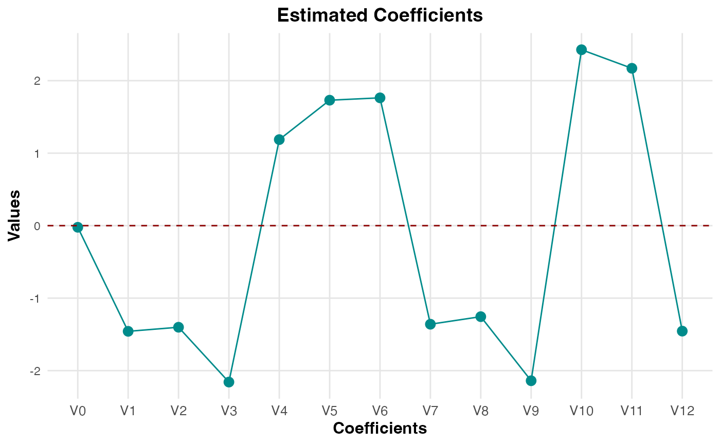
- Estimated Coefficients
Generates a line plot with points for the estimated coefficients of the regression model. If an intercept term is included in the model, it will be labeled as
beta_0. Otherwise, the coefficients are labeled sequentially asbeta_1,beta_2, etc., based on the covariates. This plot helps to visualize the contribution of each predictor variable to the model. Iflabel = TRUE, numeric values are displayed.- Risk Contributions
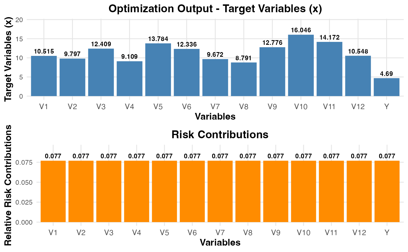
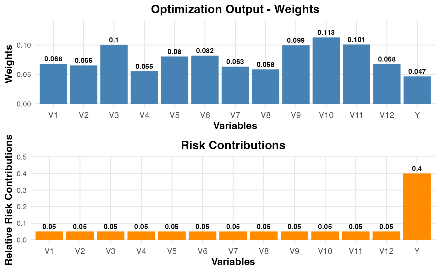
If the model includes a risk parity component, the function will check if the optimization results (e.g.,
orp_fit$weightsfor the budget method, ororp_fit$xfor the target method, along withorp_fit$relativeRiskContrib) are available. If available, two bar plots are created:Optimization Variables: A bar plot that visualizes the optimal variables assigned to each covariate and the response variable (weights for budget, target parameters for target).
Risk Contributions: A bar plot that visualizes the relative risk contributions of each covariate and the response variable.
If
label = TRUE, numeric labels are added above the bars for clarity. If they are not found, a warning is issued.
Author
Ziwei Chen, Vali Asimit and Pietro Millossovich
Maintainer: Ziwei Chen <ziwei.chen.3@citystgeorges.ac.uk>
Examples
# Example usage for `savvyPR` with Correlated Data:
set.seed(123)
n <- 100
p <- 12
# Create highly correlated predictors to demonstrate parity regression
base_var <- rnorm(n)
x <- matrix(rnorm(n * p, sd = 0.1), n, p) + base_var
beta <- matrix(rnorm(p), p, 1)
y <- x %*% beta + rnorm(n, sd = 0.5)

# Fit a Budget-based parity regression model
result_budget <- savvyPR(x, y, method = "budget", val = 0.05, intercept = TRUE)
plot(result_budget, plot_type = "estimated_coefficients", label = FALSE)

plot(result_budget, plot_type = "risk_contributions", label = TRUE)


# Fit a Target-based parity regression model
result_target <- savvyPR(x, y, method = "target", val = 1, intercept = TRUE)
plot(result_target, plot_type = "risk_contributions", label = TRUE)
# Fit a Target-based parity regression model
result_target <- savvyPR(x, y, method = "target", val = 1, intercept = TRUE)
plot(result_target, plot_type = "risk_contributions", label = TRUE)