Savvy Parity Regression Model Estimation with 'savvyPR'
Source:vignettes/savvyPR_example.Rmd
savvyPR_example.RmdIntroduction
This vignette demonstrates how to use the savvyPR
package for parity regression model estimation and cross-validation. The
package handles multicollinearity by applying risk parity constraints,
supporting both Budget-based and Target-based parameterizations.
Installation
# Install the development version from GitHub
# devtools::install_github("Ziwei-ChenChen/savvyPR)
library(savvyPR)
library(MASS)
library(glmnet)
## Loading required package: Matrix## Loaded glmnet 4.1-8Parity Regression Model Estimation
The savvyPR function is used to fit a parity regression
model. Here we demonstrate its usage with synthetic, highly correlated
data.
library(MASS)
library(glmnet)

# Function to create a correlation matrix for X
create_corr_matrix <- function(rho, p) {
  corr_matrix <- diag(1, p)
  for (i in 2:p) {
    for (j in 1:(i-1)) {
      corr_matrix[i, j] <- rho^(abs(i - j))
      corr_matrix[j, i] <- corr_matrix[i, j] # symmetric matrix
    }
  }
  return(corr_matrix)
}

# Function to generate beta values with both positive and negative signs
generate_beta <- function(p) {
  half_p <- ceiling(p / 2)
  beta <- rep(c(1, -1), length.out = p) * rep(1:half_p, each = 2)[1:p]
  return(beta)
}

set.seed(123)
n <- 1500
p <- 15
rho <- -0.5

corr_matrix <- create_corr_matrix(rho, p)
x <- mvrnorm(n = n, mu = rep(0, p), Sigma = corr_matrix)
beta <- generate_beta(p + 1)
sigma_vec <- abs(rnorm(n = n, mean = 15, sd = sqrt(1)))
y <- rnorm(n, mean = as.vector(cbind(1,x)%*%beta), sd = sigma_vec)

# 1. Run OLS estimation with intercept
result_ols <- lm(y ~ x)
coef_ols <- coef(result_ols)

# 2. Run Ridge Regression (RR) estimation
result_RR <- glmnet(x, y, alpha = 0, lambda = 1)
coef_RR <- coef(result_RR)

# 3. Run PR estimation (Budget Method)
result_pr_budget <- savvyPR(x, y, method = "budget", val = 0.05, intercept = TRUE)
print(result_pr_budget)
##
## Call: savvyPR(x = x, y = y, method = "budget", val = 0.05, intercept = TRUE)
##
## Method Number of Non-Zero Coefficients Intercept Included Lambda Value
## budget 16 Yes NA
##
## Coefficients:
## Coefficient Estimate
## (Intercept) 0.9474
## X1 -3.6223
## X2 3.7272
## X3 -3.4870
## X4 4.1283
## X5 -4.1596
## X6 5.1385
## X7 -4.9644
## X8 6.0606
## X9 -6.0015
## X10 6.3743
## X11 -5.6775
## X12 7.8006
## X13 -7.3068
## X14 9.0372
## X15 -8.7735
coef_pr_budget <- coef(result_pr_budget)

# 4. Run PR estimation (Target Method)
result_pr_target <- savvyPR(x, y, method = "target", val = 1, intercept = TRUE)
print(result_pr_target)
##
## Call: savvyPR(x = x, y = y, method = "target", val = 1, intercept = TRUE)
##
## Method Number of Non-Zero Coefficients Intercept Included Lambda Value
## target 16 Yes NA
##
## Coefficients:
## Coefficient Estimate
## (Intercept) 0.9978
## X1 -4.1012
## X2 4.1303
## X3 -3.8591
## X4 4.4168
## X5 -4.5009
## X6 5.4143
## X7 -5.2861
## X8 6.2761
## X9 -6.2403
## X10 6.5827
## X11 -5.9788
## X12 7.9785
## X13 -7.5766
## X14 9.2430
## X15 -9.0638
coef_pr_target <- coef(result_pr_target)

# Calculate the L2 distance to true beta
ols_L2 <- sqrt(sum((beta - coef_ols)^2))
print(paste("OLS L2:", ols_L2))
## [1] "OLS L2: 2.24654287653346"## [1] "Ridge L2: 2.10076303047981"## [1] "PR Budget L2: 4.6582202853575"## [1] "PR Target L2: 5.74454449168347"You can use the summary function to get detailed
statistics for your models:
summary(result_pr_budget)## Summary of Parity Model
## ===================================================================
##
## Parameterization Method: budget
## Intercept: Included
##
## Call:
## savvyPR(x = x, y = y, method = "budget", val = 0.05, intercept = TRUE)
##
## Residuals:
## 0% 25% 50% 75% 100%
## -56.4721096 -10.9724126 -0.1952992 10.8910982 48.9682405
##
## Coefficients:
## Estimate Std. Error t value Pr(>|t|) 2.5 % 97.5 % Signif.
## (Intercept) 0.9474 0.431 2.1984 0.0281 0.1028 1.7921 *
## X1 -3.6223 0.5026 -7.2072 9.0577e-13 -4.6073 -2.6372 ***
## X2 3.7272 0.5477 6.8045 1.4663e-11 2.6536 4.8007 ***
## X3 -3.487 0.5593 -6.2346 5.8903e-10 -4.5832 -2.3908 ***
## X4 4.1283 0.55 7.5065 1.0423e-13 3.0504 5.2062 ***
## X5 -4.1596 0.5612 -7.4125 2.0734e-13 -5.2595 -3.0598 ***
## X6 5.1385 0.5528 9.2957 5.0478e-20 4.0551 6.2219 ***
## X7 -4.9644 0.5569 -8.914 1.4106e-18 -6.056 -3.8729 ***
## X8 6.0606 0.5498 11.0227 3.2671e-27 4.983 7.1383 ***
## X9 -6.0015 0.5598 -10.7216 6.9524e-26 -7.0986 -4.9044 ***
## X10 6.3743 0.5607 11.3678 9.0139e-29 5.2753 7.4733 ***
## X11 -5.6775 0.5529 -10.2685 6.0457e-24 -6.7612 -4.5938 ***
## X12 7.8006 0.5748 13.5718 1.2278e-39 6.6741 8.9272 ***
## X13 -7.3068 0.5552 -13.1595 1.7263e-37 -8.3951 -6.2185 ***
## X14 9.0372 0.5627 16.059 1.2454e-53 7.9342 10.1401 ***
## X15 -8.7735 0.4755 -18.4495 1.3655e-68 -9.7056 -7.8415 ***
## ---
## Signif. codes: 0 '***' 0.001 '**' 0.01 '*' 0.05 '.' 0.1 ' ' 1
##
## Residual standard error: 16.6436 on 1484 degrees of freedom
## Multiple R-squared: 0.7826 , Adjusted R-squared: 0.7804
## F-statistic: 356.1532 on 15 and 1484 DF, p-value: 0.0000e+00
## AIC: 8451.993 , BIC: 8537.004 , Deviance: 411082.4
summary(result_pr_target)## Summary of Parity Model
## ===================================================================
##
## Parameterization Method: target
## Intercept: Included
##
## Call:
## savvyPR(x = x, y = y, method = "target", val = 1, intercept = TRUE)
##
## Residuals:
## 0% 25% 50% 75% 100%
## -58.9781373 -11.4050252 -0.2897816 11.4442435 52.0560037
##
## Coefficients:
## Estimate Std. Error t value Pr(>|t|) 2.5 % 97.5 % Signif.
## (Intercept) 0.9978 0.4524 2.2056 0.0276 0.1111 1.8844 *
## X1 -4.1012 0.5276 -7.7736 1.4166e-14 -5.1352 -3.0671 ***
## X2 4.1303 0.575 7.1833 1.0728e-12 3.0033 5.2572 ***
## X3 -3.8591 0.5871 -6.5731 6.8054e-11 -5.0098 -2.7084 ***
## X4 4.4168 0.5773 7.6507 3.5751e-14 3.2853 5.5484 ***
## X5 -4.5009 0.5891 -7.6408 3.8518e-14 -5.6555 -3.3464 ***
## X6 5.4143 0.5803 9.3308 3.6947e-20 4.277 6.5516 ***
## X7 -5.2861 0.5846 -9.042 4.6833e-19 -6.4319 -4.1402 ***
## X8 6.2761 0.5772 10.8739 1.4943e-26 5.1448 7.4073 ***
## X9 -6.2403 0.5876 -10.6202 1.9152e-25 -7.392 -5.0887 ***
## X10 6.5827 0.5886 11.1835 6.2051e-28 5.4291 7.7364 ***
## X11 -5.9788 0.5804 -10.3013 4.4033e-24 -7.1163 -4.8412 ***
## X12 7.9785 0.6033 13.2239 8.0385e-38 6.796 9.1611 ***
## X13 -7.5766 0.5829 -12.9991 1.1453e-36 -8.7189 -6.4342 ***
## X14 9.243 0.5907 15.647 3.3967e-51 8.0853 10.4008 ***
## X15 -9.0638 0.4992 -18.1572 1.0869e-66 -10.0422 -8.0854 ***
## ---
## Signif. codes: 0 '***' 0.001 '**' 0.01 '*' 0.05 '.' 0.1 ' ' 1
##
## Residual standard error: 17.4711 on 1484 degrees of freedom
## Multiple R-squared: 0.7605 , Adjusted R-squared: 0.758
## F-statistic: 314.0652 on 15 and 1484 DF, p-value: 0.0000e+00
## AIC: 8597.558 , BIC: 8682.57 , Deviance: 452975.2The package also provides built-in plotting functions to visualize the coefficients and the risk parity optimization distributions.
# Plot the estimated coefficients
plot(result_pr_budget, plot_type = "estimated_coefficients", label = TRUE)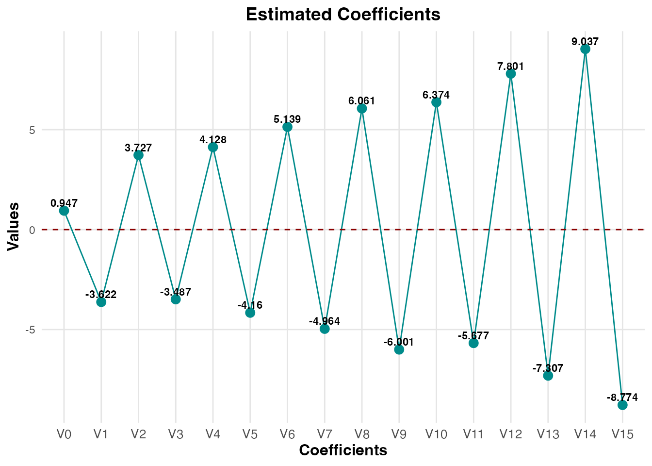
plot(result_pr_target, plot_type = "estimated_coefficients", label = FALSE)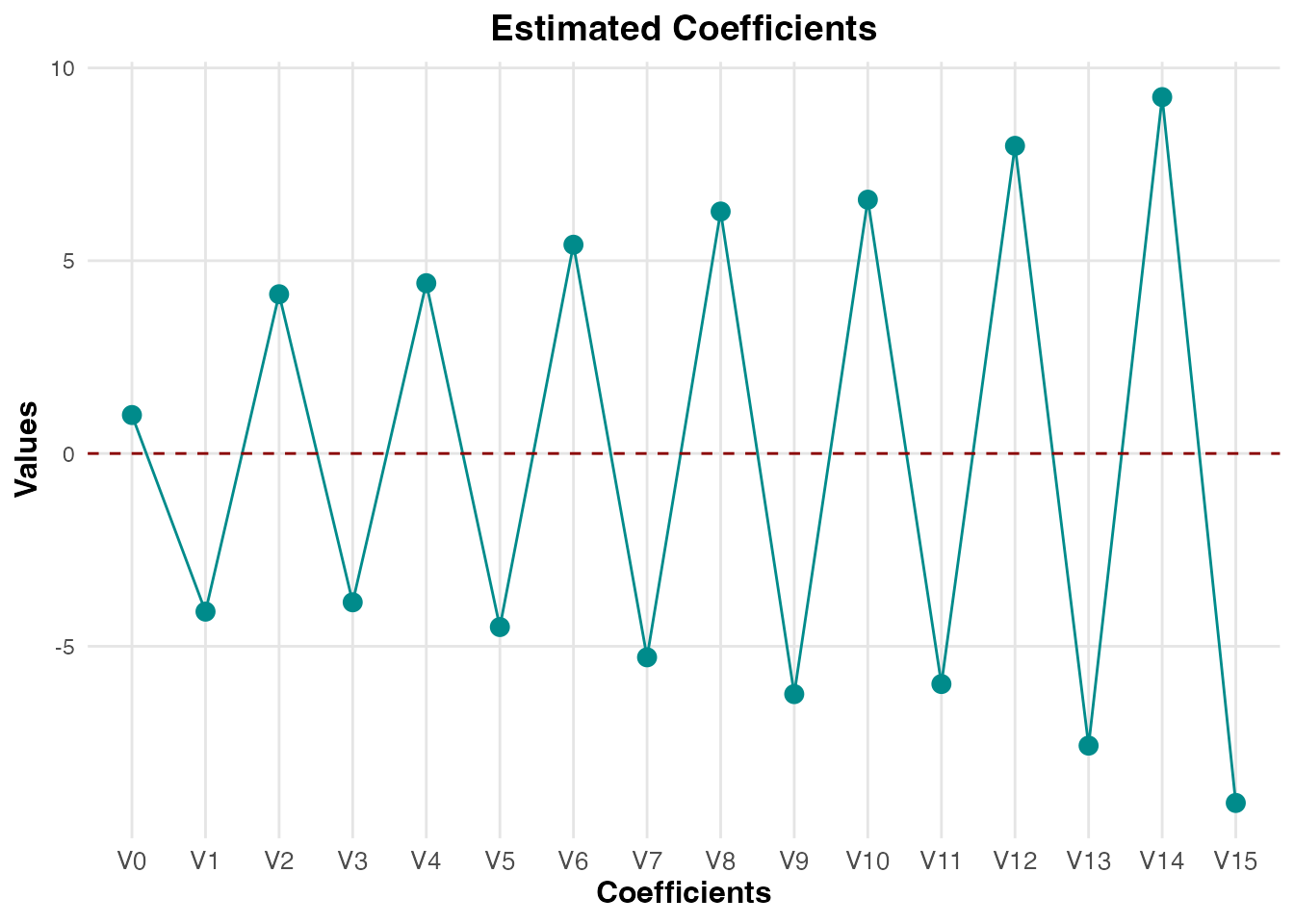
# Plot the risk contributions and weights/target variables
plot(result_pr_budget, plot_type = "risk_contributions", label = TRUE)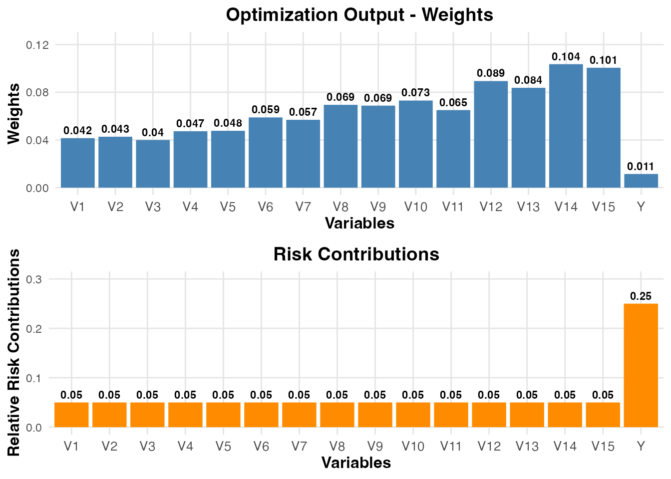
plot(result_pr_target, plot_type = "risk_contributions", label = FALSE)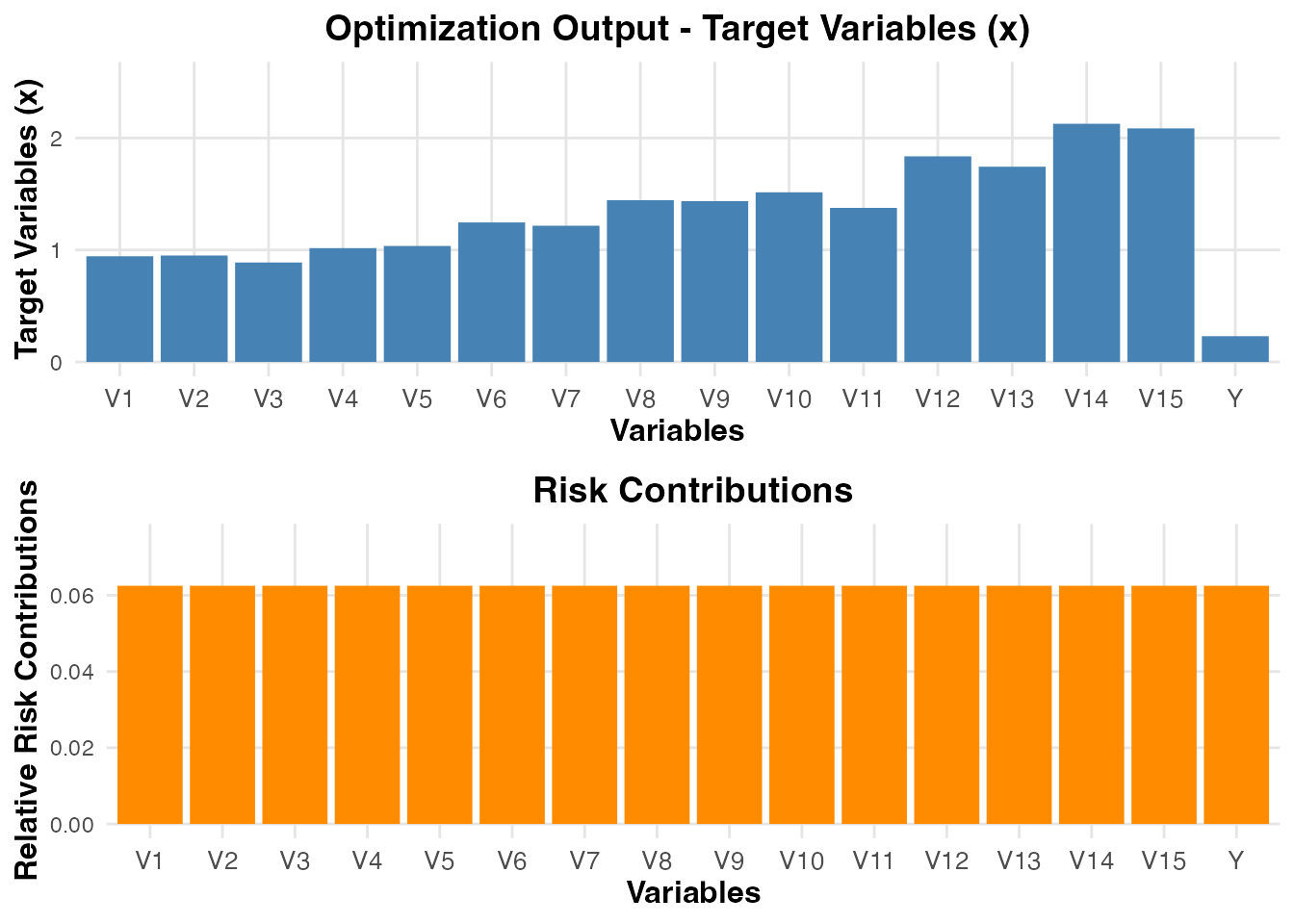
Cross-Validation for Parity Regression Models
The cv.savvyPR function performs cross-validation to
select optimal parameters. It handles both the “budget” sequence and the
“target” sequence automatically.
# Cross-validation with Ridge
result_rr_cv <- cv.glmnet(x, y, alpha = 0, folds = 5)
fit_rr1 <- glmnet(x, y, alpha = 0, lambda = result_rr_cv$lambda.min)
coef_rr_cv <- coef(fit_rr1)[,1]

# Cross-validation with model type PR1 (Budget Method)
result_pr_cv1 <- cv.savvyPR(x, y, method = "budget", folds = 5, model_type = "PR1", measure_type = "mse")
coef_pr_cv1 <- coef(result_pr_cv1)

# Cross-validation with model type PR2 (Target Method)
result_pr_cv2 <- cv.savvyPR(x, y, method = "target", folds = 5, model_type = "PR2", measure_type = "mse")
coef_pr_cv2 <- coef(result_pr_cv2)

# Cross-validation with model type PR3 (Budget Method)
result_pr_cv3 <- cv.savvyPR(x, y, method = "budget", folds = 5, model_type = "PR3", measure_type = "mse")
coef_pr_cv3 <- coef(result_pr_cv3)

# Calculate the L2 distance
print(paste("Ridge CV L2:", sqrt(sum((beta - coef_rr_cv)^2))))
## [1] "Ridge CV L2: 2.02357341480252"## [1] "PR1 CV (Budget) L2: 2.13653233706683"## [1] "PR2 CV (Target) L2: 2.13123848154008"## [1] "PR3 CV (Budget) L2: 1.95028924294646"We can summarize the cross-validation results to see the optimal tuning values chosen by the algorithm.
summary(result_pr_cv1)## Summary of Cross-Validated Parity Model
## ===================================================================
##
## Parameterization Method: budget
## Intercept: Included
##
## Call:
## cv.savvyPR(x = x, y = y, method = "budget", folds = 5, model_type = "PR1",
## measure_type = "mse")
##
## Residuals:
## 0% 25% 50% 75% 100%
## -48.7354673 -10.2964301 -0.2204747 10.6115532 52.7232048
##
## Coefficients:
## Estimate Std. Error t value Pr(>|t|) 2.5 % 97.5 % Signif.
## (Intercept) 0.7757 0.3938 1.9699 0.0490 0.0039 1.5476 *
## X1 -1.4127 0.4593 -3.0759 0.0021 -2.3128 -0.5125 **
## X2 2.366 0.5005 4.727 2.4950e-06 1.385 3.347 ***
## X3 -1.7786 0.5111 -3.4801 0.0005 -2.7803 -0.7769 ***
## X4 3.533 0.5026 7.0302 3.1358e-12 2.5481 4.518 ***
## X5 -2.7157 0.5128 -5.296 1.3616e-07 -3.7208 -1.7107 ***
## X6 4.5448 0.5051 8.9974 6.8876e-19 3.5548 5.5348 ***
## X7 -3.7245 0.5089 -7.3185 4.0907e-13 -4.7219 -2.727 ***
## X8 5.5978 0.5024 11.1415 9.5942e-28 4.6131 6.5826 ***
## X9 -5.2052 0.5115 -10.1763 1.4707e-23 -6.2077 -4.2027 ***
## X10 5.9252 0.5124 11.5639 1.1254e-29 4.921 6.9295 ***
## X11 -4.5194 0.5052 -8.9451 1.0806e-18 -5.5096 -3.5291 ***
## X12 7.4844 0.5252 14.2501 2.7928e-43 6.455 8.5138 ***
## X13 -6.4236 0.5074 -12.6604 5.8619e-35 -7.4181 -5.4292 ***
## X14 8.5038 0.5142 16.537 1.6420e-56 7.496 9.5117 ***
## X15 -7.9255 0.4345 -18.2386 3.2262e-67 -8.7772 -7.0738 ***
## ---
## Signif. codes: 0 '***' 0.001 '**' 0.01 '*' 0.05 '.' 0.1 ' ' 1
##
## Residual standard error: 15.2088 on 1484 degrees of freedom
## Multiple R-squared: 0.8185 , Adjusted R-squared: 0.8166
## F-statistic: 446.0718 on 15 and 1484 DF, p-value: 0.0000e+00
## AIC: 8181.532 , BIC: 8266.543 , Deviance: 343259.3
##
## Cross-Validation Summary:
## Mean Cross-Validation Error ( mse: Mean-Squared Error ): 234.5913
## Optimal Val: 0.002051
## Fixed Lambda: 0
summary(result_pr_cv2)## Summary of Cross-Validated Parity Model
## ===================================================================
##
## Parameterization Method: target
## Intercept: Included
##
## Call:
## cv.savvyPR(x = x, y = y, method = "target", folds = 5, model_type = "PR2",
## measure_type = "mse")
##
## Residuals:
## 0% 25% 50% 75% 100%
## -49.3945508 -10.3670298 -0.2395204 10.7127881 54.4065137
##
## Coefficients:
## Estimate Std. Error t value Pr(>|t|) 2.5 % 97.5 % Signif.
## (Intercept) 0.764 0.3937 1.9405 0.0525 -0.0077 1.5356 .
## X1 -1.1001 0.4592 -2.396 0.0167 -2.0001 -0.2002 *
## X2 2.3507 0.5004 4.6976 2.8764e-06 1.3699 3.3315 ***
## X3 -1.5982 0.511 -3.1279 0.0018 -2.5997 -0.5968 **
## X4 3.5608 0.5024 7.087 2.1112e-12 2.576 4.5455 ***
## X5 -2.605 0.5127 -5.0812 4.2258e-07 -3.6098 -1.6002 ***
## X6 4.4804 0.505 8.8718 2.0229e-18 3.4906 5.4702 ***
## X7 -3.6559 0.5088 -7.1855 1.0567e-12 -4.6531 -2.6587 ***
## X8 5.5172 0.5023 10.9836 4.8790e-27 4.5327 6.5017 ***
## X9 -5.1496 0.5114 -10.0701 4.0618e-23 -6.1519 -4.1474 ***
## X10 5.8444 0.5123 11.4088 5.8468e-29 4.8404 6.8485 ***
## X11 -4.4766 0.5051 -8.8625 2.1904e-18 -5.4666 -3.4866 ***
## X12 7.381 0.5251 14.0566 3.1557e-42 6.3518 8.4102 ***
## X13 -6.3708 0.5073 -12.5592 1.8691e-34 -7.365 -5.3766 ***
## X14 8.3905 0.5141 16.3204 3.3696e-55 7.3829 9.3982 ***
## X15 -7.7903 0.4344 -17.9316 3.0955e-65 -8.6418 -6.9388 ***
## ---
## Signif. codes: 0 '***' 0.001 '**' 0.01 '*' 0.05 '.' 0.1 ' ' 1
##
## Residual standard error: 15.2052 on 1484 degrees of freedom
## Multiple R-squared: 0.8186 , Adjusted R-squared: 0.8167
## F-statistic: 446.3271 on 15 and 1484 DF, p-value: 0.0000e+00
## AIC: 8180.829 , BIC: 8265.841 , Deviance: 343098.6
##
## Cross-Validation Summary:
## Mean Cross-Validation Error ( mse: Mean-Squared Error ): 234.9548
## Optimal Val: 0
## Fixed Lambda: 0.7543
summary(result_pr_cv3)## Summary of Cross-Validated Parity Model
## ===================================================================
##
## Parameterization Method: budget
## Intercept: Included
##
## Call:
## cv.savvyPR(x = x, y = y, method = "budget", folds = 5, model_type = "PR3",
## measure_type = "mse")
##
## Residuals:
## 0% 25% 50% 75% 100%
## -49.1703575 -10.3073085 -0.3193037 10.8172768 53.4727869
##
## Coefficients:
## Estimate Std. Error t value Pr(>|t|) 2.5 % 97.5 % Signif.
## (Intercept) 0.7686 0.3939 1.9513 0.0512 -0.0034 1.5405 .
## X1 -1.4104 0.4593 -3.0704 0.0022 -2.3107 -0.5101 **
## X2 2.2843 0.5006 4.5631 5.4569e-06 1.3032 3.2655 ***
## X3 -1.8217 0.5112 -3.5638 0.0004 -2.8236 -0.8199 ***
## X4 3.4573 0.5026 6.8782 8.9074e-12 2.4721 4.4424 ***
## X5 -2.7309 0.5129 -5.3246 1.1674e-07 -3.7361 -1.7257 ***
## X6 4.4236 0.5052 8.7558 5.4115e-18 3.4334 5.4138 ***
## X7 -3.7275 0.509 -7.3232 3.9544e-13 -4.7252 -2.7299 ***
## X8 5.479 0.5025 10.903 1.1107e-26 4.4941 6.4639 ***
## X9 -5.1863 0.5116 -10.1376 2.1323e-23 -6.189 -4.1836 ***
## X10 5.803 0.5125 11.3233 1.4394e-28 4.7986 6.8075 ***
## X11 -4.5692 0.5053 -9.042 4.6805e-19 -5.5596 -3.5788 ***
## X12 7.2898 0.5253 13.8772 2.9219e-41 6.2602 8.3194 ***
## X13 -6.4111 0.5075 -12.6334 7.9892e-35 -7.4057 -5.4164 ***
## X14 8.3162 0.5143 16.1692 2.7349e-54 7.3081 9.3242 ***
## X15 -7.7702 0.4346 -17.8779 6.8380e-65 -8.622 -6.9183 ***
## ---
## Signif. codes: 0 '***' 0.001 '**' 0.01 '*' 0.05 '.' 0.1 ' ' 1
##
## Residual standard error: 15.2115 on 1484 degrees of freedom
## Multiple R-squared: 0.8184 , Adjusted R-squared: 0.8166
## F-statistic: 445.8784 on 15 and 1484 DF, p-value: 0.0000e+00
## AIC: 8182.064 , BIC: 8267.075 , Deviance: 343381.1
##
## Cross-Validation Summary:
## Mean Cross-Validation Error ( mse: Mean-Squared Error ): 234.3193
## Fixed Val: 0.002051
## Optimal Lambda: 0.03728We can also visualize the cross-validated models:
# Plot coefficients and risk contributions for PR1
plot(result_pr_cv1, plot_type = "estimated_coefficients", label = TRUE)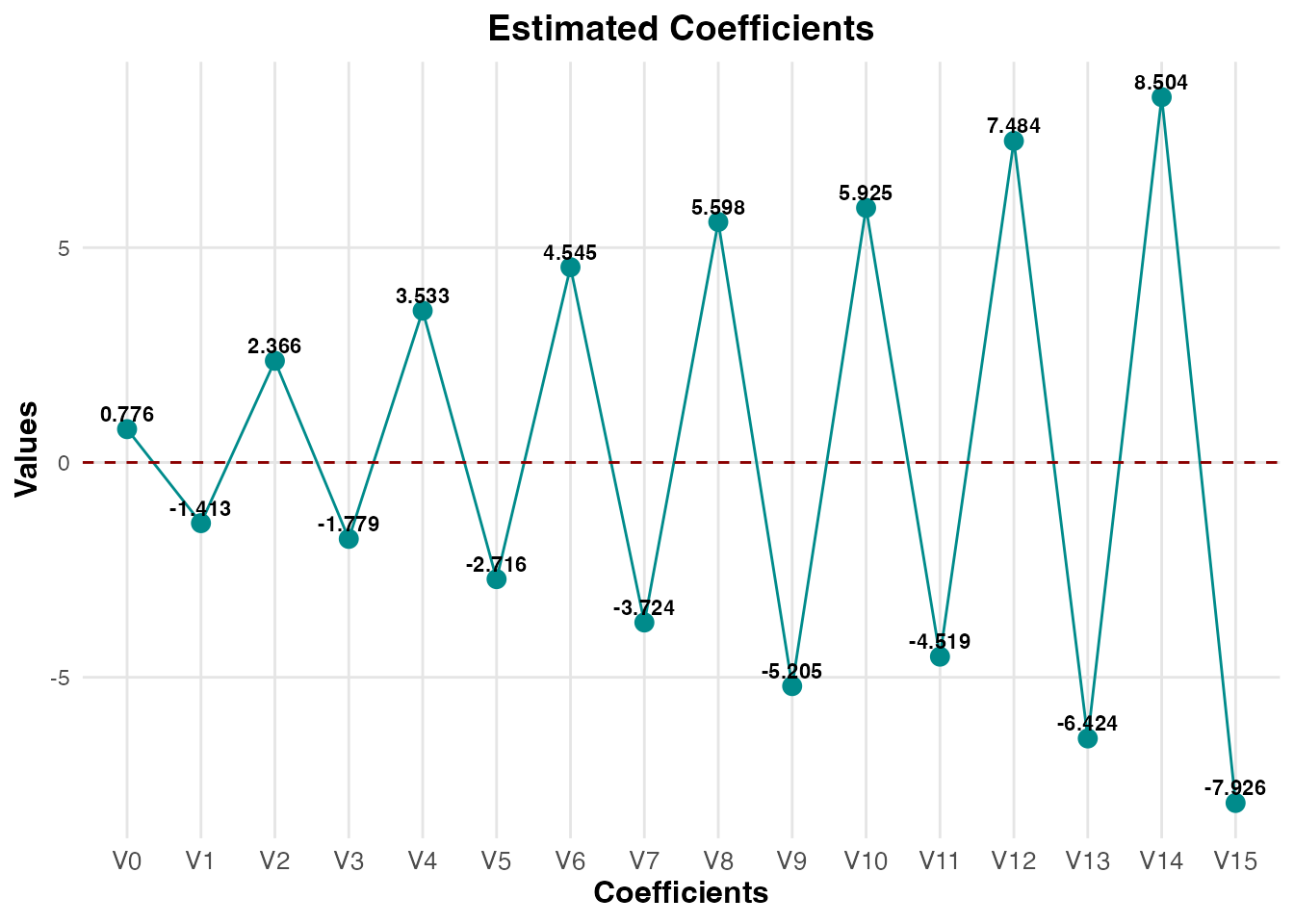
plot(result_pr_cv1, plot_type = "risk_contributions",label = TRUE)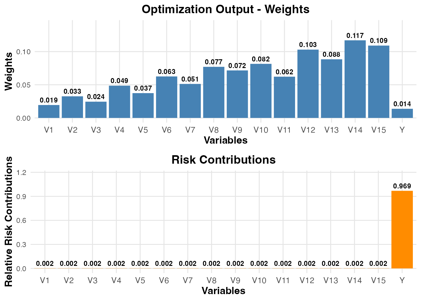
# Plot coefficients and risk contributions for PR2
plot(result_pr_cv2, plot_type = "estimated_coefficients", label = FALSE)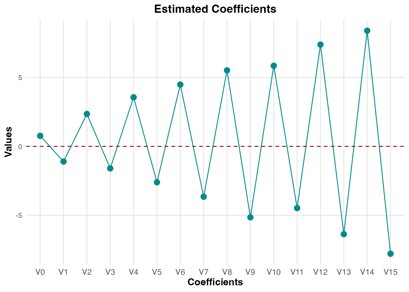
# Cannot plot risk-contribution for PR2 since the tuning parameter val=0 is fixed.
#plot(result_pr_cv2, plot_type = "risk_contributions", label = FALSE)
We can visualize the cross-validation error curves to see exactly where the optimal minimum was found.
# Plot the cross-validation errors for each model
plot(result_rr_cv)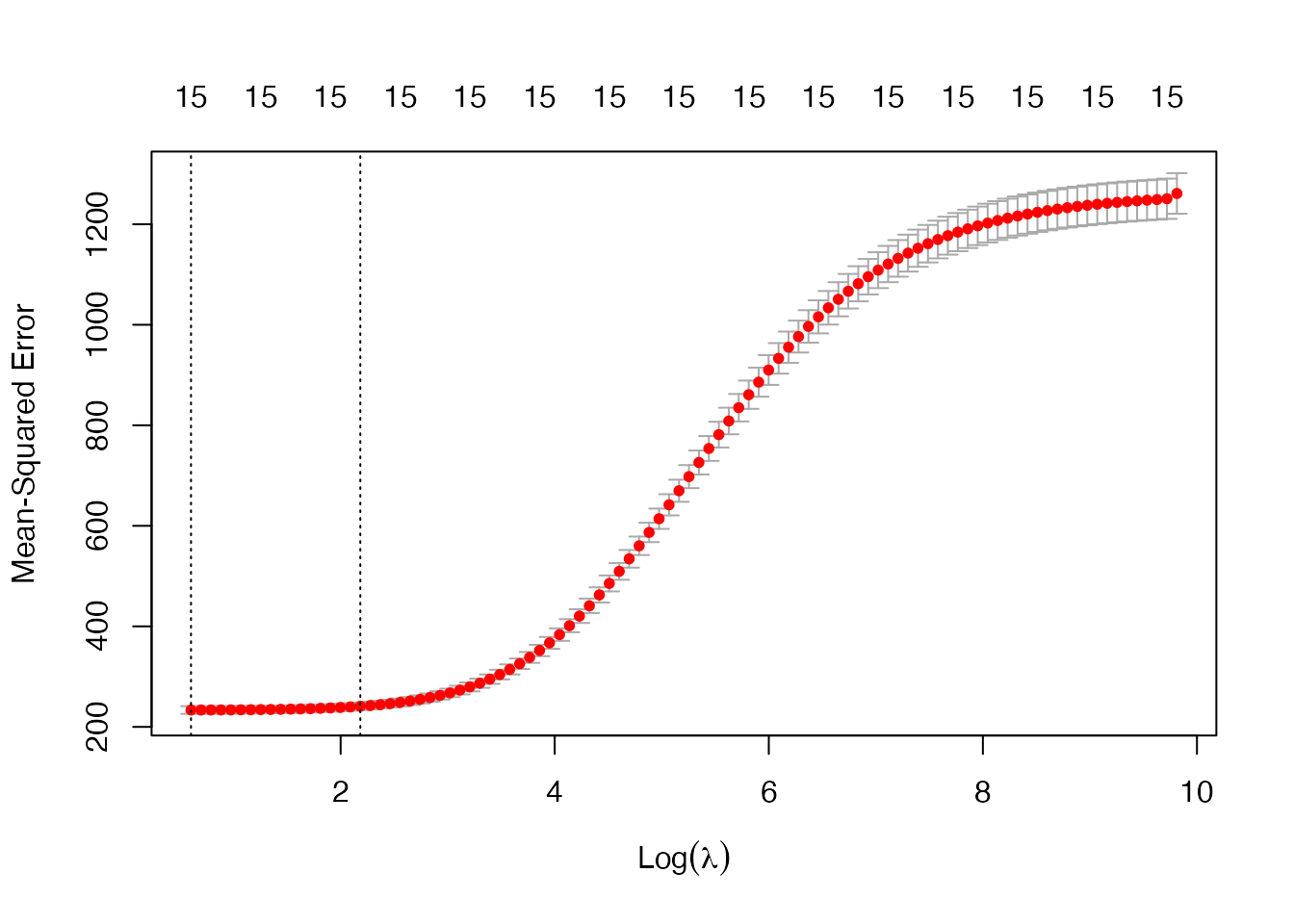
plot(result_pr_cv1, plot_type = "cv_errors", label = TRUE)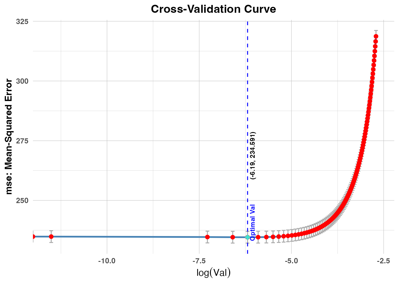
plot(result_pr_cv2, plot_type = "cv_errors")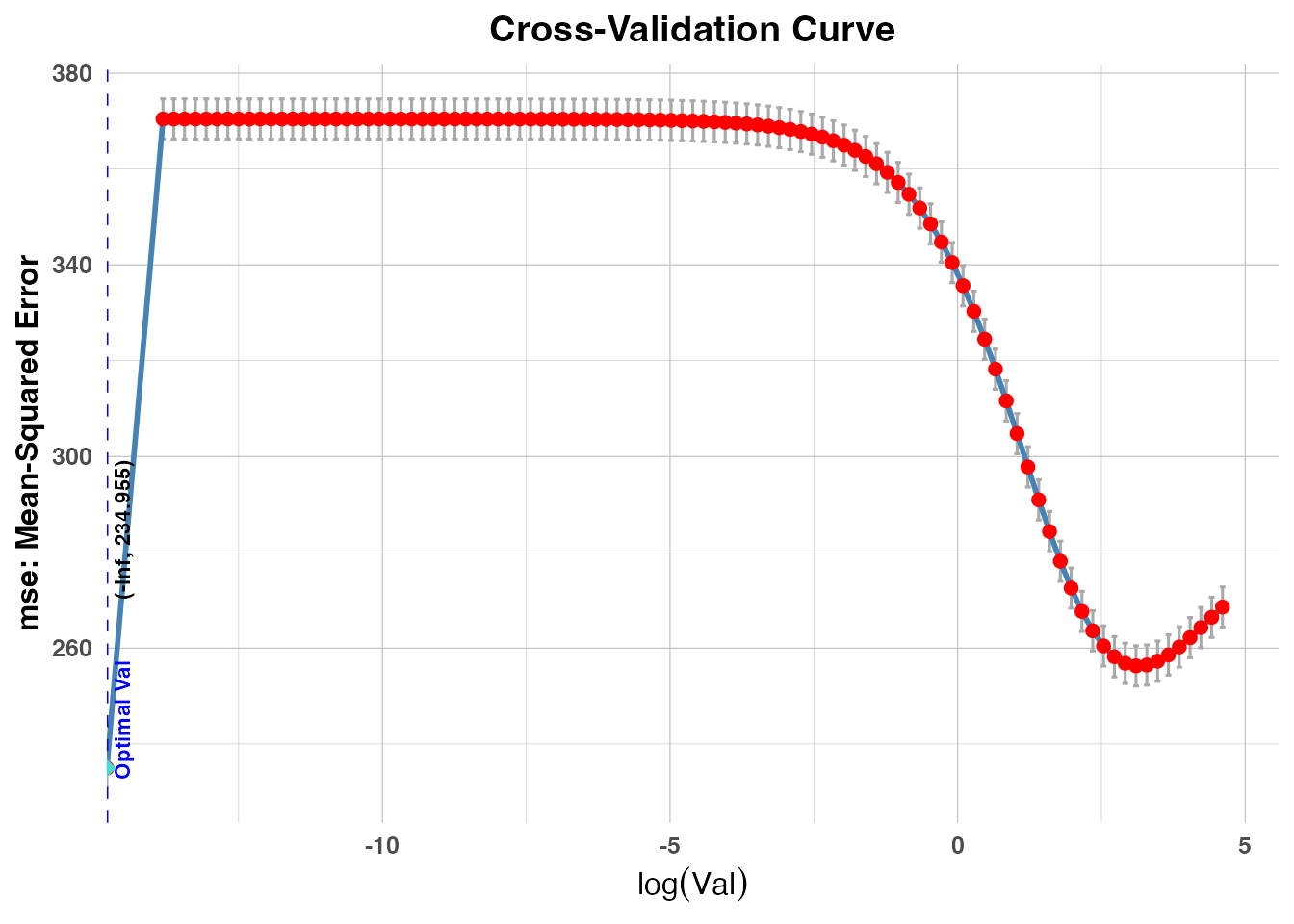
plot(result_pr_cv3, plot_type = "cv_errors", label = FALSE)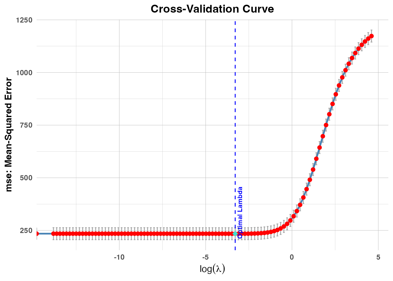
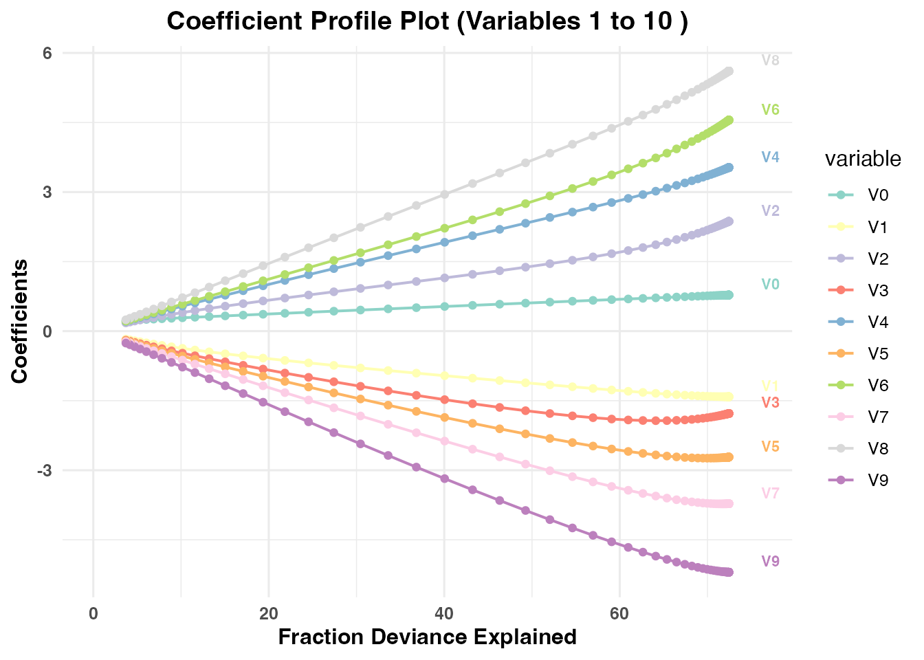
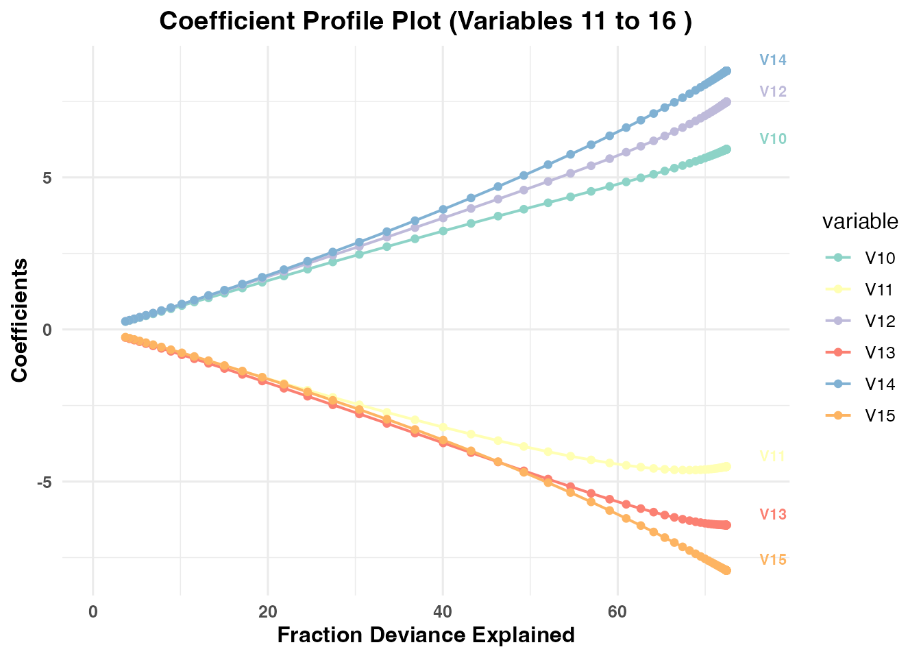
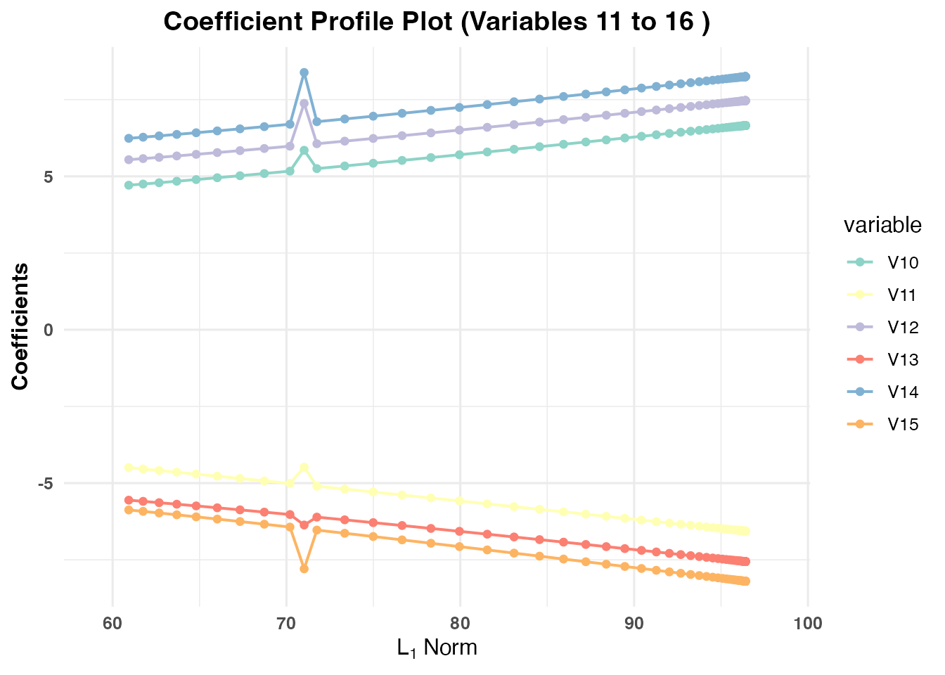
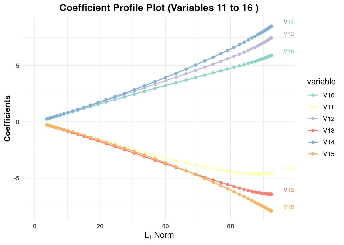
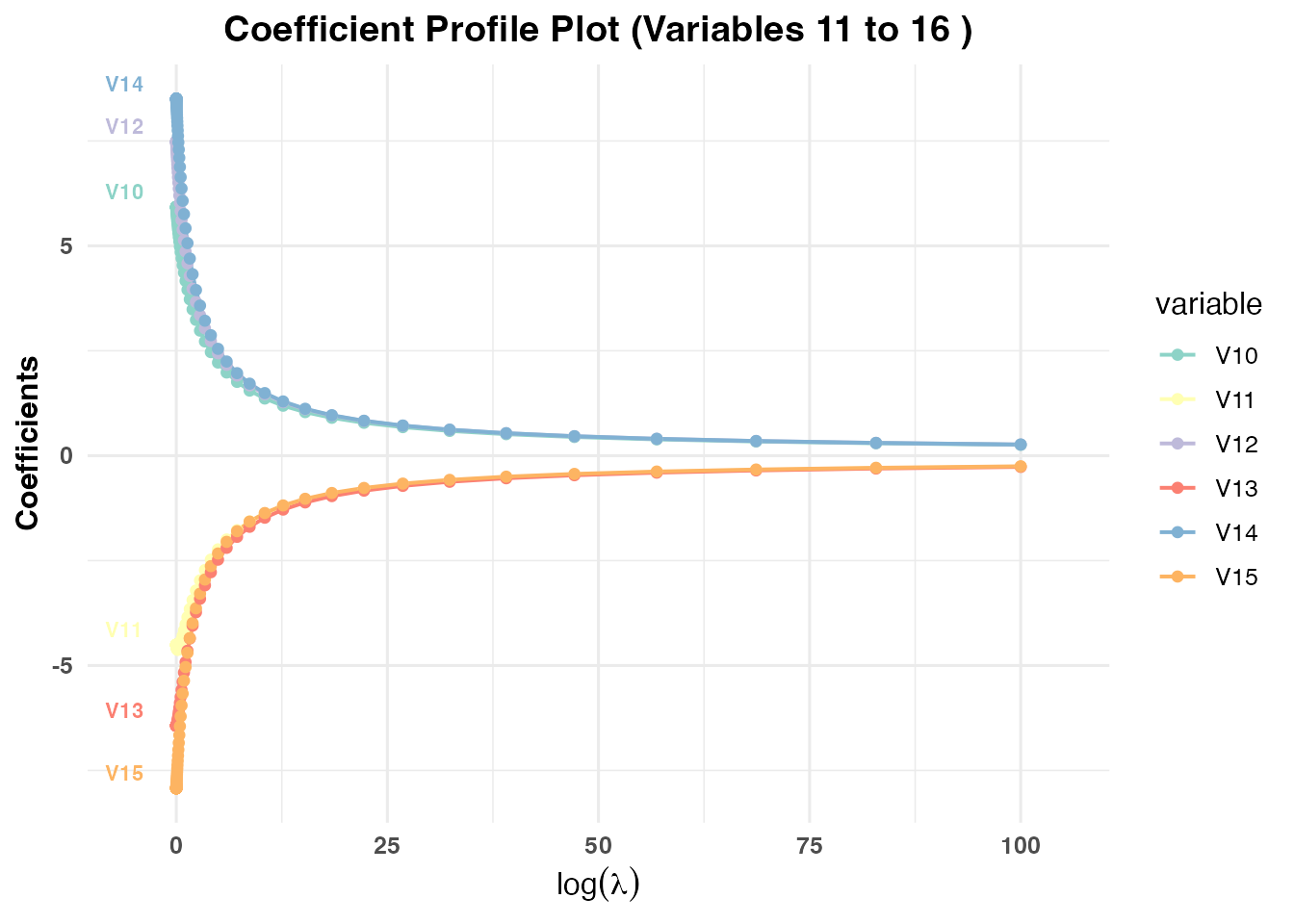
Finally, we can plot the Coefficient Paths to see how the coefficients shrink or change as the tuning parameter varies. Notice that we use xvar = “val” to plot against the unified tuning parameter.
# Plot the coefficient paths for cross-validation models
plot(result_pr_cv1, plot_type = "cv_coefficients", xvar = "val", max_vars_per_plot = 10, label = TRUE)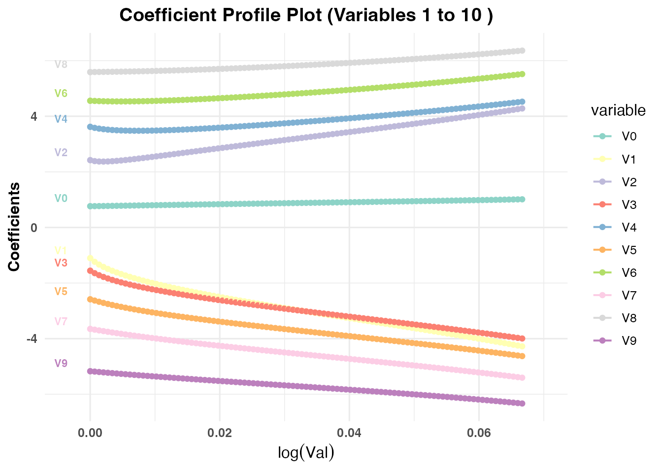
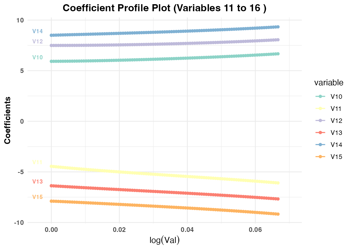
# Show what happens when max_vars_per_plot exceeds the limit (will trigger a warning and reset to 10)
plot(result_pr_cv2, plot_type = "cv_coefficients", xvar = "norm", max_vars_per_plot = 12, label = FALSE)
## Warning in plotCVCoef(result_list = x, label = label, xvar = xvar,
## max_vars_per_plot = max_vars_per_plot, : max_vars_per_plot cannot exceed 10.
## Setting max_vars_per_plot to 10.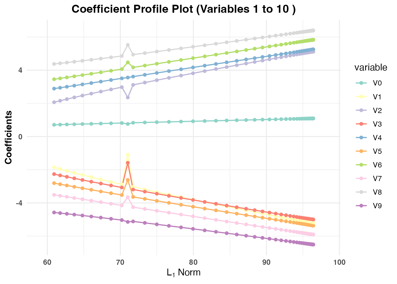
# PR3 uses dual-optimization, so we can plot against lambda as well
plot(result_pr_cv3, plot_type = "cv_coefficients", xvar = "norm", max_vars_per_plot = 10, label = TRUE)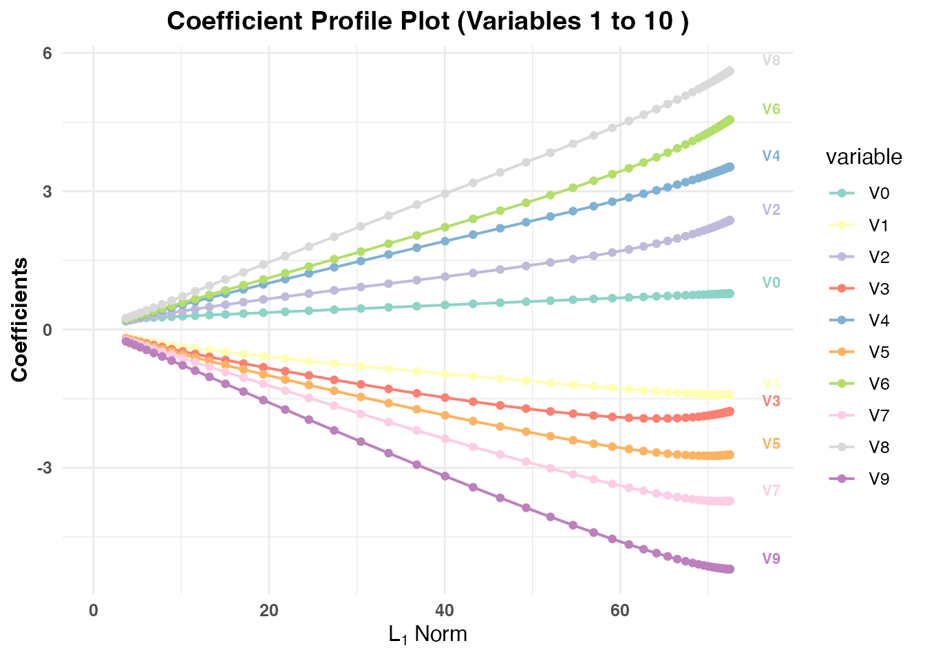
plot(result_pr_cv3, plot_type = "cv_coefficients", xvar = "lambda", max_vars_per_plot = 10, label = TRUE)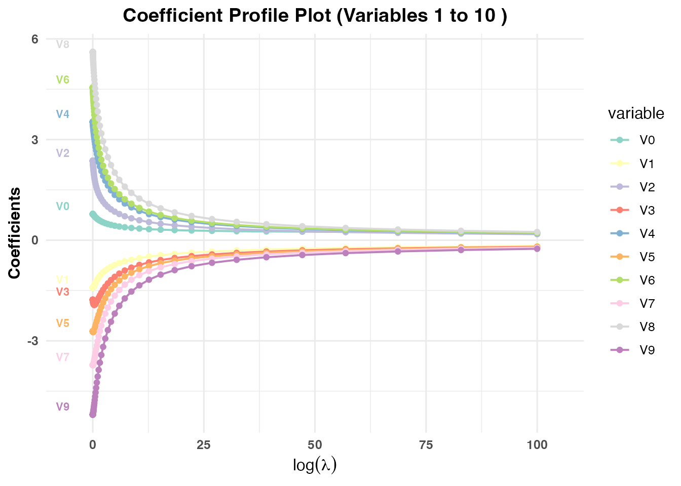
plot(result_pr_cv3, plot_type = "cv_coefficients", xvar = "dev", max_vars_per_plot = 10, label = TRUE)